- 참고 블로그
CRF란?
- 영상보다는 자연어처리 분야에서 많이 사용되는 통계적 모델링 기법입니다.
- 사진 하나의 행동을 분류할 때, 하나의 행동 Sequence만을 보고 판단하지 않고 사진을 찍은 순간의 이전/이후를 참조하여 지금 상태를 결정합니다.
머신러닝/딥러닝, 리눅스, 소프트웨어, 그리고 일상
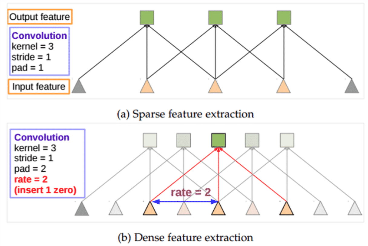
같은 Kernel size의 컨볼루션을 한 번만 수행하면, Stride의 수를 늘린것과 동일하게 Feature가 작아지는 효과가 있고 이와 동시에 Receptive Field의 크기가 확장되는 효과를 얻을 수 있습니다.
Atrous Convolution은 기존 Wavelet을 이용한 신호분석에 사용되던 방식이지만, 이를 영상과 같은 2차원 데이터에도 활용하여 연산량을 줄이는 효과를 얻을 수 있습니다.

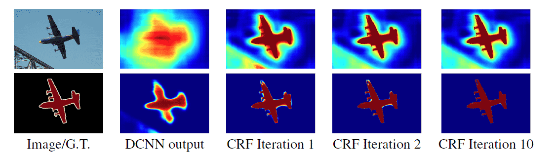
DeepLab V1에서는 Atrous convolution과 함께 CRF를 후처리 과정으로 사용해 예측 정확도를 높혔습니다. 기존 Short-Range CRF는 Segmentation noise를 없애는 용도로 사용되었는데, 전체 픽셀에 대한 Fully-Connected CRF을 수행할 경우 높은 정확도로 Segmentation이 가능한 것으로 알려져 Fully-Connected CRF를 수행하였습니다.
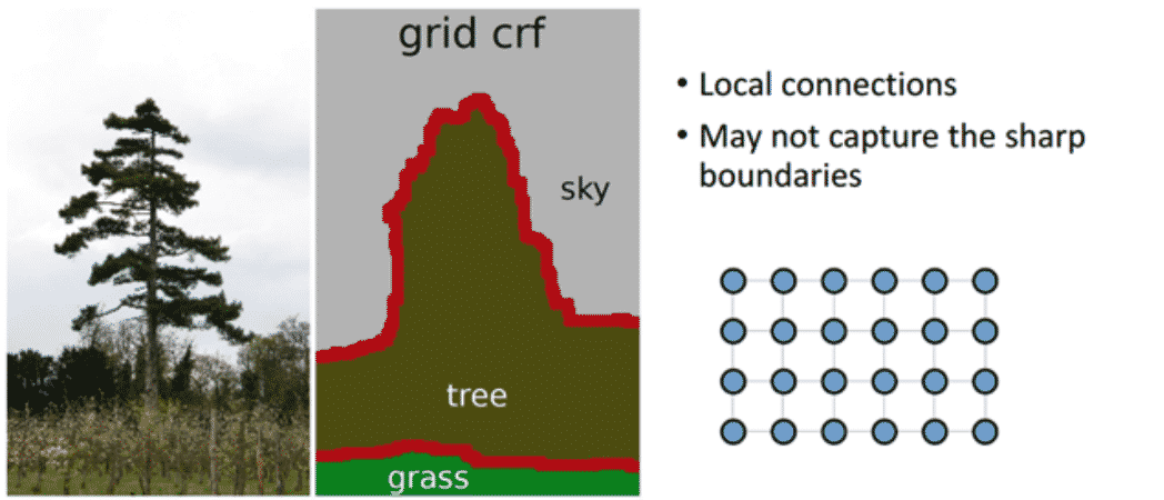
기존의 Short-range CRF의 경우 Local connection (Neighbor-) 정보만을 사용하게 되므로 오히려 Segmentation이 뭉뚱그려지고, Sharp한 boundary보다는 Noise에 강인한 결과를 얻을 수 있었습니다.

이를 Fully-Connected CRF (추후 DeepLab V3에서는 DenseCRF라고 불립니다)를 이용하여 Pixel-by-pixel로 Fully Connected Graph로 연결합니다. 물론 노드의 수가 상당히 많은 Markov Chain이므로 시간이 상당히 오래 걸리는 Task인데, DenseCRF 논문에서는 이를 Mean Field Approximation이라는 방법으로 해결하였습니다. 이 방식을 적용하여 Message passing을 이용한 iteration 방식을 이용하면, 효과적(효율적)으로 DenseCRF를 수행할 수 있게 됩니다.
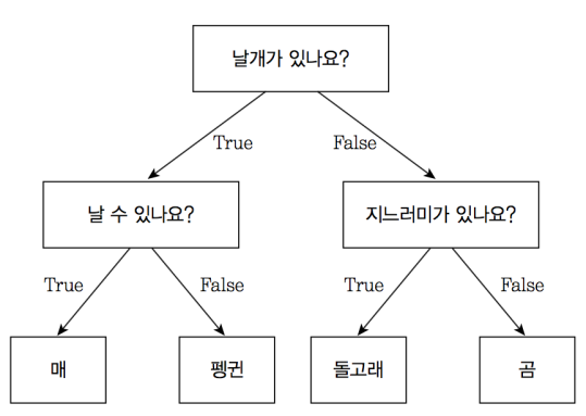
Decision Tree는 특정 질문에 따라 데이터를 구분하는 모델입니다. 분기마다 항상 변수 영역을 두 개로 구분하는 Binary Tree의 형태를 가집니다. 트리의 기본 구조에 따라 첫 노드(=첫 질문)은 Root Node, 마지막 질문(=마지막 노드)는 Terminal Node(Leaf Node)라고 합니다.
깊이가 깊어질수록 의사 결정에 따른 데이터가 나뉘게 됩니다.


다만 지나치게 깊은 의사결정트리로 데이터를 구분하게 되거나 결정 트리에 아무 Parameter도 주지 않고 모델링을 할 경우 오버피팅이 발생합니다.
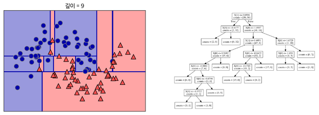
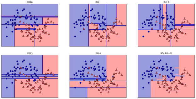
결정 트리를 만들 때, 많은 Feature를 이용하게 되면 그만큼 가지가 많아지고 이는 오버피팅이 발생하는 원인이 됩니다. 이 Feature 중 랜덤으로 n개만 선택해서 결정 트리를 만드는 과정을 m번 반복하여, m개의 결정 트리를 만들 수 있습니다(예를 들어, 30가지의 Feature 중 랜덤으로 5가지를 뽑아서 결정트리를 만드는 과정을 5번 반복할 수 있습니다). 이러한 여러 개의 결정 트리들의 예측값들 중 가장 많이 나온 값 하나를 최종적으로 선택합니다. 이러한 결과 선택 과정을 앙상블(Ensemble)이라고 합니다. (블로그에서 가장 와닿었던 대목은, “문제를 풀 때 한명의 똑똑한 사람보다 100명의 평범한 사람들이 더 잘 푼다”라는 부분이었습니다.)
위 사진에서 아래쪽 최우측에 있는 그림이 랜덤 포레스트의 Decision Boundary입니다. 나머지는 총 5개의 결정 트리 각각의 Decision Boundary를 보여줍니다.
Tensorflow on RTX 3000 series (RTX 3070, RTX 3080, RTX 3090)
OS: Windows 10 Education (Build 19042.608)
Architecture: x86_64 (amd64)
Git branch: v2.4.0-rc0
Python: 3.7 (anaconda)
Target CUDA and CUDNN: CUDA 11.1 Update 1, CUDNN v8.0.5 (Novemvber 9th, 2020) (requires login)
Target arch: CC 8.6, 6.1 → Must be also usable on GTX 1000 series!
Numpy: 1.19.4 (Must be manually reinstalled back to version 1.19.3 before using!)
pip install tensorflow-2.4.0rc0-cp37-cp37m-win_amd64.whlpip install numpy==1.19.3# Memory Pre-configuration
config = tf.compat.v1.ConfigProto(
gpu_options=tf.compat.v1.GPUOptions(
per_process_gpu_memory_fraction=0.8,
allow_growth = True
)
# device_count = {'GPU': 1}
)
session = tf.compat.v1.Session(config=config)
tf.compat.v1.keras.backend.set_session(session)An Introduction to different Types of Convolutions in Deep Learning을 번역한 글입니다. 개인 공부를 위해 번역해봤으며 이상한 부분은 언제든 알려주세요 🙂
Convolution의 여러 유형에 대해 빠르게 소개하며 각각의 장점을 알려드리겠습니다. 단순화를 위해서, 이 글에선 2D Convolution에만 초점을 맞추겠습니다
우선 convolutional layer을 정의하기 위한 몇개의 파라미터를 알아야 합니다
2D convolution using a kernel size of 3, stride of 1 and padding
역자 : 파란색이 input이며 초록색이 output입니다
(a.k.a. atrous convolutions)
2D convolution using a 3 kernel with a dilation rate of 2 and no padding
Dilated Convolution은 Convolutional layer에 또 다른 파라미터인 dilation rate를 도입했습니다. dilation rate은 커널 사이의 간격을 정의합니다. dilation rate가 2인 3×3 커널은 9개의 파라미터를 사용하면서 5×5 커널과 동일한 시야(view)를 가집니다.
5×5 커널을 사용하고 두번째 열과 행을 모두 삭제하면 (3×3 커널을 사용한 경우 대비)동일한 계산 비용으로 더 넓은 시야를 제공합니다.
Dilated convolution은 특히 real-time segmentation 분야에서 주로 사용됩니다. 넓은 시야가 필요하고 여러 convolution이나 큰 커널을 사용할 여유가 없는 경우 사용합니다
역자 : Dilated Convolution은 필터 내부에 zero padding을 추가해 강제로 receptive field를 늘리는 방법입니다. 위 그림에서 진한 파란 부분만 weight가 있고 나머지 부분은 0으로 채워집니다. (receptive field : 필터가 한번 보는 영역으로 사진의 feature를 추출하기 위해선 receptive field가 높을수록 좋습니다)
pooling을 수행하지 않고도 receptive field를 크게 가져갈 수 있기 때문에 spatial dimension 손실이 적고 대부분의 weight가 0이기 때문에 연산의 효율이 좋습니다. 공간적 특징을 유지하기 때문에 Segmentation에서 많이 사용합니다
(a.k.a. deconvolutions or fractionally strided convolutions)
어떤 곳에선 deconvolution이라는 이름을 사용하지만 실제론 deconvolution이 아니기 때문에 부적절합니다. 상황을 악화시키기 위해 deconvolution이 존재하지만, 딥러닝 분야에선 흔하지 않습니다. 실제 deconvolution은 convolution의 과정을 되돌립니다. 하나의 convolutional layer에 이미지를 입력한다고 상상해보겠습니다. 이제 출력물을 가져와 블랙 박스에 넣으면 원본 이미지가 다시 나타납니다. 이럴 경우 블랙박스가 deconvolution을 수행한다고 할 수 있습니다. 이 deconvolution이 convolutional layer가 수행하는 것의 수학적 역 연산입니다.
역자 : 왜 deconvolution이 아닌지는 링크에 나와있습니다
Transposed Convolution은 deconvolutional layer와 동일한 공간 해상도를 생성하기 점은 유사하지만 실제 수행되는 수학 연산은 다릅니다. Transposed Convolutional layer는 정기적인 convolution을 수행하며 공간의 변화를 되돌립니다.
2D convolution with no padding, stride of 2 and kernel of 3
혼란스러울 수 있으므로 구체적인 예를 보겠습니다. convolution layer에 넣을 5×5 이미지가 있습니다. stride는 2, padding은 없고 kernel은 3×3입니다. 이 결과는 2×2 이미지가 생성됩니다.
이 과정을 되돌리고 싶다면, 역 수학 연산을 위해 input의 각 픽셀으로부터 9개의 값을 뽑아야 합니다. 그 후에 우리는 stride가 2인 출력 이미지를 지나갑니다. 이 방법이 deconvolution입니다
Transposed 2D convolution with no padding, stride of 2 and kernel of 3
transposed convolution은 위와 같은 방법을 사용하지 않습니다. deconvolution과 공통점은 convolution 작업을 하면서 5×5 이미지의 output을 생성하는 것입니다. 이 작업을 하기 위해 input에 임의의 padding을 넣어야 합니다.
상상할 수 있듯, 이 단계에선 위의 과정을 반대로 수행하지 않습니다.
단순히 이전 공간 해상도를 재구성하고 convolution을 수행합니다. 수학적 역 관계는 아니지만 인코더-디코더 아키텍쳐의 경우 유용합니다. 이 방법은 2개의 별도 프로세스를 진행하는 것 대신 convolution된 이미지의 upscaling을 결합할 수 있습니다
역자 : Transposed Convolution는 일반적인 convolution을 반대로 수행하고 싶은 경우에 사용하며, 커널 사이에 0을 추가합니다
위 그림은 일반적인 convolution 연산을 행렬로 표현한 것입니다
transposed convolution 연산을 행렬로 표현한 것입니다. 첫 이미지의 sparse 매트릭스 C를 inverse해서 우변(Y output)에 곱해줍니다. 그러면 Input의 값을 구할 수 있습니다.
정리하면 전치(transpose)하여 우변에 곱해주기 때문에 transposed convolution이라 부릅니다.
Up-sampling with Transposed Convolution 번역 글을 참고하시면 명쾌하게 이해가 될거에요! Convolution Operation은 input values와 output values 사이에 공간 연결성을 가지고 있습니다. 3×3 kernel을 사용한다면, 9개의 values가(kernel) 1개의 value(output, 문지른 후의 결과물)와 연결됩니다. 따라서 many to one 관계라고 볼 수 있습니다
Transposed Convolution은 1개의 value를 9개의 values로 변경합니다. 이것은 one to many 관계라고 볼 수 있습니다.
(2019년 9월) 역자 : 위 convolution 매트릭스 연산의 그림에 오류가 있습니다. 한번 어떤 부분이 오류인지 생각해보신 후, 답이 궁금하시면 댓글을 확인해주세요 🙂 제보해주신 정종원님, 김남욱님 감사합니다
separable convolution에선 커널 작업을 여러 단계로 나눌 수 있습니다. convolution을 y = conv(x, k)로 표현해봅시다. x는 입력 이미지, y는 출력 이미지, k는 커널입니다. 그리고 k=k1.dot(k2)로 계산된다고 가정해보겠습니다. 이것은 K와 2D convolution을 수행하는 대신 k1와 k2로 1D convolution하는 것과 동일한 결과를 가져오기 때문에 separable convolution이 됩니다.
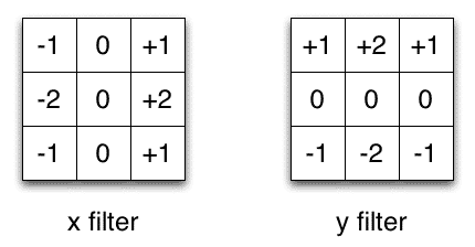
Sobel X and Y filters
이미지 처리에서 자주 사용되는 Sobel 커널을 예로 들겠습니다. 벡터 [1, 0, -1]과 [1, 2, 1].T를 곱하면 동일한 커널을 얻을 수 있습니다. 동일 작업을 하기 위해 9개의 파라미터 대신 6개가 필요합니다. 이 사례는 Spatial Separable Convolution의 예시이지만, 딥러닝에선 사용되지 않습니다
수정 : 사실 1xN, Nx1 커널 레이어를 쌓아 Separable convolution과 유사한 것을 만들 수 있습니다. 이것은 최근 유망한 결과를 보여준 EffNet라는 아키텍쳐에서 사용되었습니다.
뉴럴넷에선 depthwise separable convolution라는 것을 주로 사용합니다. 이 방법은 채널을 분리하지 않고 spatial convolution을 수행한 다음 depthwise convolution을 수행합니다. 예를 들어보겠습니다.
16개의 input 채널과 32개의 output 채널에 3×3 convolutional 레이어가 있다고 가정하겠습니다. 16개의 채널마다 32개의 3×3 커널이 지나가며 512(16*32)개의 feature map이 생성됩니다. 그 다음, 모든 입력 채널에서 1개의 feature map을 병합하여 추가합니다. 32번 반복하면 32개의 output 채널을 얻을 수 있습니다.
같은 예제에서 depthwise separable convolution을 위해 1개의 3×3 커널로 16 채널을 탐색해 16개의 feature map을 생성합니다. 합치기 전에 32개의 1×1 convolution으로 16개의 featuremap을 지나갑니다. 결과적으로 위에선 4068(163233) 매개 변수를 얻는 반면 656(1633 + 163211) 매개변수를 얻습니다
이 예는 depthwise separable convolution(depth multiplier가 1이라고 불리는)것을 구체적으로 구현한 것입니다. 이런 layer에서 가장 일반적인 형태입니다.
우리는 spatial하고 depthwise한 정보를 나눌 수 있다는 가정하에 이 작업을 합니다. Xception 모델의 성능을 보면 이 이론이 효과가 있는 것으로 보입니다. depthwise seprable convolution은 매개변수를 효율적으로 사용하기 때문에 모바일 장치에도 사용됩니다
역자 : 채널, 공간상 상관성 분리를 하는 인셉션 모델을 극단적으로 밀어붙여 depthwise separable convolution 구조를 만듭니다. input의 1×1 convolution을 씌운 후 나오는 모든 채널에 3×3 convolution을 수행합니다. 원글에서 separable convolution의 설명이 부족한 것 같아 PR12의 영상을 보고 이해했습니다
유재준님의 PR-034: Inception and Xception과 이진원님의 PR-044: MobileNet을 보면 이해가 잘됩니다 🙂
이것으로 여러 종류의 convolution 여행을 끝내겠습니다. Convolution에 대한 짧은 요약을 가지고가길 바라며 남아있는 질문은 댓글을 남겨주시고, 더 많은 convolution 애니메이션이 있는 Github를 확인해주세요
COCO 데이터셋 Annotation에 대한 설명을 해 주신 글이 있어, 스크랩해 보았다.
Annotation 파일은 한 줄짜리 json 형식으로 되어 있습니다. 혹시라도, 이 파일을 그냥 vi로 열면 안됩니다. 수백메가 크기의 한 줄 짜리 파일이라, vi가 감당을 못합니다. 그래서, json beautifier를 이용하여 줄바꿈을 해 주어야 분석이 쉽습니다.
https://stedolan.github.io/jq/에서 jq binary를 다운로드 받습니다. 저는 64-bit Ubuntu용으로 다운로드 받아서, 파일 이름이 jq-linux64 네요. 그 다음,
$ jq-linux64 . instances_val2017.json > instances_val2017.beautified.json
이와 같이 하면 줄바꿈이 적용된 JSON 파일인 instances_val2017.beautified.json 파일이 생성됩니다.
이 중에서 instances에 대해 좀 더 자세히 알아보겠습니다.
Instances json file의 첫 부분은 아래와 같이 information과 license의 종류에 대한 내용입니다.
{
  "info": {
    "description": "COCO 2017 Dataset",
    "url": "http://cocodataset.org",
    "version": "1.0",
    "year": 2017,
    "contributor": "COCO Consortium",
    "date_created": "2017/09/01"
  },
  "licenses": [
    {
      "url": "http://creativecommons.org/licenses/by-nc-sa/2.0/",
      "id": 1,
      "name": "Attribution-NonCommercial-ShareAlike License"
    },
    ...
  ],
그 다음엔, 그림 파일에 대한 내용이 나옵니다.
  "images": [
    ...
    {
      "license": 1,
      "file_name": "000000324158.jpg",
      "coco_url": "http://images.cocodataset.org/val2017/000000324158.jpg",
      "height": 334,
      "width": 500,
      "date_captured": "2013-11-19 23:54:06",
      "flickr_url": "http://farm1.staticflickr.com/169/417836491_5bf8762150_z.jpg",
      "id": 324158
    },
    ...
  ],
그 다음엔, 각 그림에 대한 annotation 정보가 나옵니다. Annotation이란, 그림에 있는 사물/사람의 segmentation mask와 box 영역, 카테고리 등의 정보를 말합니다. 아래 예는 COCO API Demo에서 사용된 image인 324159 그림의 annotation 중 일부 입니다.
  "annotations": [
    ...
    {
      "segmentation": [
        [
          216.7,
          211.89,
          216.16,
          217.81,
          215.89,
          220.77,

          ...
          212.16
        ]
      ],
      "area": 759.3375500000002,
      "iscrowd": 0,
      "image_id": 324158,
      "bbox": [
        196.51,
        183.36,
        23.95,
        53.02
      ],
      "category_id": 18,
      "id": 10673
    },
    ...
    {
      "segmentation": [
        [
          44.2,
          167.74,
          48.39,
          162.71,
          ...
          167.58
        ]
      ],
      "area": 331.9790999999998,
      "iscrowd": 0,
      "image_id": 324158,
      "bbox": [
        44.2,
        161.19,
        36.78,
        13.78
      ],
      "category_id": 3,
      "id": 345846
    },
    ...
  ],
마지막으로, category 리스트가 나옵니다.
  "categories": [
    {
      "supercategory": "person",
      "id": 1,
      "name": "person"
    },
    ...
  ]
}The new Tensorflow 2.0 is going to standardize on Keras as its High-level API. The existing Keras API will mostly remain the same, while Tensorflow features like eager execution, distributed training and other deeper Tensorflow integration will be added or improved. I think it’s a good time to revisit Keras as someone who had switched to use PyTorch most of the time.
I wrote an article benchmarking the TPU on Google Colab with the Fashion-MNIST dataset when Colab just started to provide TPU runtime. This time I’ll use a larger dataset (CIFAR-10) and an external image augmentation library [albumentation](https://github.com/albu/albumentations)s.
It turns out that implementing a custom image augmentation pipeline is fairly easy in the newer Keras. We could give up some flexibility in PyTorch in exchange of the speed up brought by TPU, which is not yet supported by PyTorch yet.
ngrok)The notebooks are largely based on the work by Jannik Zürn described in this post:
I updated the model architecture from the official Keras example and modified some of the data preparation code.
From the Keras documentation:
[Sequence](https://keras.io/utils/)are a safer way to do multiprocessing. This structure guarantees that the network will only train once on each sample per epoch which is not the case with generators.
Most Keras tutorials use the ImageDataGenerator class to generate batch and do image augmentation. But it doesn’t leave much room for customization (unless you spend some time reading the source code and extend the class) and the augmentation toolbox might not be comprehensive or fast enough for you.
Fortunately, there’s a Sequence class (keras.utils.Sequence) in Keras that is very similar to [Dataset](https://pytorch.org/docs/stable/data.html#torch.utils.data.Dataset) class in PyTorch (although Keras doesn’t seem to have its own [DataLoader](https://pytorch.org/docs/stable/data.html#torch.utils.data.DataLoader)). We can construct our own data augmentation pipeline like this:
Note the one major difference between Sequence and Dataset is that Sequence returns an entire batch, while Dataset returns a single entry.
In this example, the data has already been read in as numpy arrays. For larger datasets, you can store paths to the image files and labels in the file system in the class constructor, and read the images dynamically in the __getitem__ method via one of the two methods:
cv2.cvtColor(cv2.imread(filepath), cv2.COLOR_RGB2BGR)np.array(Image.open(filepath))Reference: An example pipeline that uses torchvision.
Now we use albumentations to define a set of augmentations to be applied randomly to training set and a (deterministic) set for the test and validation sets:
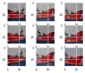
Augmented Samples
ToFloat(max_value=255) transforms the array from [0, 255] range to [0, 1] range. If you are tuning a pretrained model, you’ll want to use Normalize to set mean and std.
Just pass the sequence instances to the fit_generator method of an initialized model, Keras will do the rest for you:
By default Keras will shuffle the batches after one epoch. You can also choose to shuffle the entire dataset instead by implementing a on_epoch_end method in your Sequence class. You can also use this method to do other dynamic transformations to the dataset between epochs (as long as the __len__ stay the same, I assume).
That’s it. You now have a working customized image augmentation pipeline.
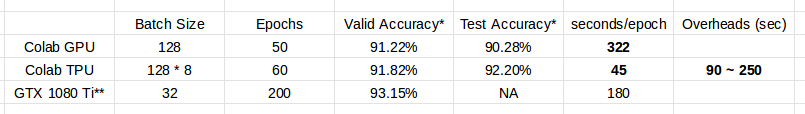
Model used: Resnet101 v2 in the official example.
Notes to the table:
[CLAHE](https://albumentations.readthedocs.io/en/latest/api/augmentations.html#albumentations.augmentations.transforms.CLAHE) op while the TPU one does not. This is due to an oversight on my part.The batch size used by Colab TPU is increased to utilize the significantly larger memory size (64GB) and TPU cores (8). Each core will received 1/8 of the batch.
Like before, one single command is enough to do the conversion:
But because the training pipeline is more complicated than the Fashion-MNIST one, I encountered a few obstacles, and had to find ways to circumvent them:
multiprocessing=True in fit_generator method, despite the fact that Sequence instances should support multiprocessing.tf.train optimizers, but on the other hand the Keras learning rate schedulers only support Keras optimizers.fit_generator call, and the compile time is fairly long and unstable (high variance between runs).The corresponding solutions:
multiprocessing=False. This one is obvious.The TPU (TPUv2 on Google Colab) greatly reduces the time needed to train an adequate model, albeit its overhead. But get ready to deal with unexpected problems since everything is really still experimental. It was really frustrating for me when the TPU backend kept crashing for no obvious reason.
The set of augmentations used here is relatively mild. There are a lot more options in the albumentations library (e.g. Cutout) for you to try.
If you found TPU working great for you, the current pricing of TPU is quite affordable for a few hours of training (Regular $4.5 per hour and preemptible $1.35 per hour). (I’m not affiliated with Google.)
In the future I’ll probably try to update the notebooks to Tensorflow 2.0 alpha or the later RC and report back anything interesting.
(This post is also published on my personal blog.)

